Why Use Genetic Programming Instead of Neural Networks?
Published:
Feature Construction with Genetic Programming for Decision Trees using Cross-Validation Loss
In the field of machine learning, feature engineering plays a crucial role. The goal of feature engineering is to construct features that are more useful for machine learning algorithms, thereby improving the performance of models. There are many methods for feature engineering, including but not limited to:
- Kernel methods: Mapping original features to higher-dimensional feature spaces to facilitate easier classification or regression. This requires the base model to have inner product operations.
- Neural networks: Using neural networks to construct new features. This requires the base model to be differentiable.
This article focuses on genetic programming (GP) for feature construction. Genetic programming is an evolutionary algorithm that optimizes solutions by simulating the process of natural selection.
In genetic programming, each solution is a program where the input is the original features and the output is the new features. Genetic programming evolves continuously to find the optimal feature construction program.
Advantages of Genetic Programming
Gradient-free optimization: Compared to kernel methods and neural networks, the advantage of genetic programming lies in its ability to optimize cross-validation error for any base learning model, rather than directly optimizing training error, which necessitates differentiability. This means genetic programming can better avoid overfitting while also being more flexible.
Symbolic representation: Unlike kernel methods and neural networks, genetic programming is based on symbolic representation, meaning the constructed features are highly interpretable.
Population optimization: Distributed search that can linearly scale to clusters. (Note: Local optima of neural networks were once considered a problem, but more and more research indicates that most critical points of neural networks are saddle points.)
Why Not Use Neural Networks?
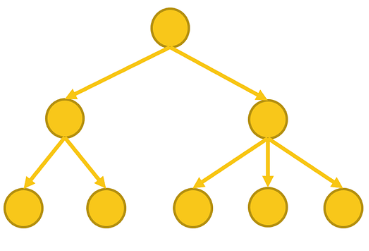
Decision Trees -> Non-differentiable -> Unable to Use Neural Networks for Feature Construction
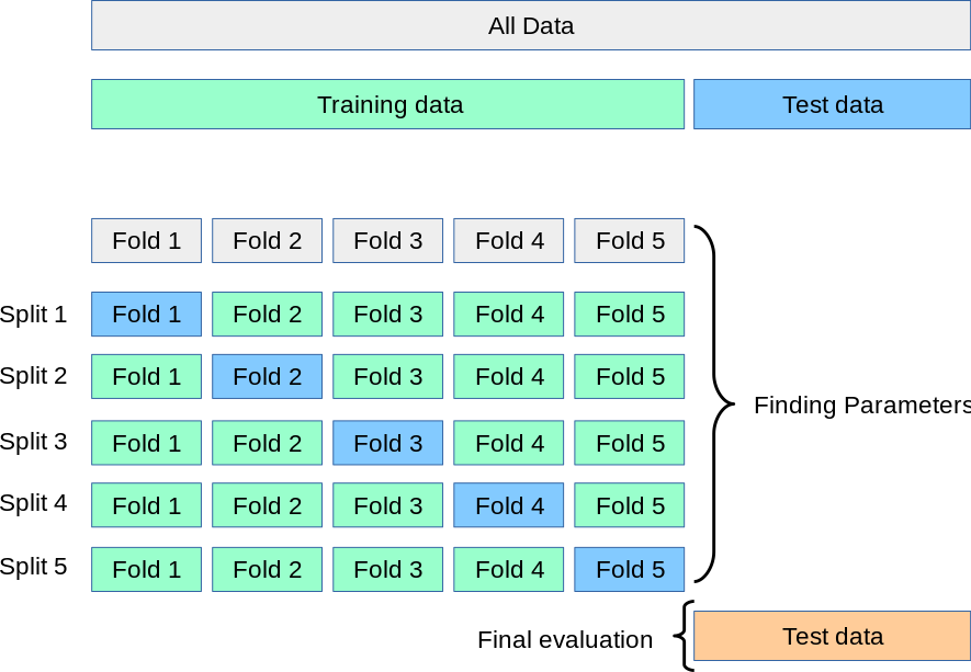
Cross-Validation Error -> Non-differentiable -> Unable to Optimize with Gradient Descent
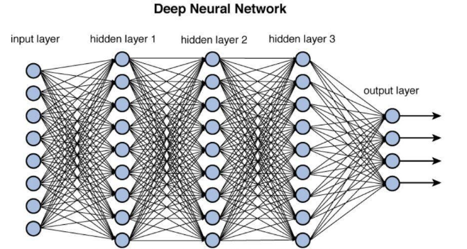
Traditional Neural Networks -> Difficult to Interpret/High Memory Consumption
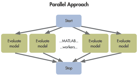
Gradient Optimization -> Difficult for Large-Scale Parallelization
Evaluation Function
As mentioned earlier, the goal of genetic programming is to optimize cross-validation error, rather than optimizing training error like traditional feature engineering methods.
It is worth noting that the cross-validation error here refers to the cross-validation error on the training set, not on the test set.
from gplearn.functions import _protected_division
from sklearn.datasets import load_iris, load_diabetes, load_breast_cancer, load_digits, load_wine
from sklearn.metrics import r2_score
from sklearn.neighbors import KNeighborsRegressor
from sklearn.model_selection import cross_val_score, train_test_split
from sklearn.pipeline import Pipeline
from sklearn.preprocessing import StandardScaler, MinMaxScaler

# Assuming we have a regression problem, with input X and output y
X, y = load_diabetes(return_X_y=True)
train_X, test_X, train_y, test_y = train_test_split(X, y, test_size=0.2, random_state=0)
scaler = StandardScaler()
train_X = scaler.fit_transform(train_X)
test_X = scaler.transform(test_X)


# The objective of solving the problem is to maximize regression cross-validation scores
def evalFeatureEngineering(individuals):
    # Create new features
    new_features = []
    for ind_num, ind in enumerate(individuals):
        func = gp.compile(expr=ind, pset=pset)
        new_features.append([func(*record) for record in train_X])

    # Transpose the new feature array
    new_features = np.transpose(np.array(new_features))

    # Use decision tree for regression
    model = DecisionTreeRegressor(min_samples_leaf=10)

    # Use cross-validation to compute error
    scores = cross_val_score(model, new_features, train_y, cv=5)

    # Return the average score
    return scores.mean(),
Representation of Multi-Tree GP Individuals
For feature construction, each GP individual can be a list of trees, where each individual contains multiple features, and each tree represents a new feature.
import operator
import random
import numpy as np
from deap import base, creator, tools, gp, algorithms
from sklearn.tree import DecisionTreeRegressor

np.random.seed(0)
random.seed(0)

def _protected_division(x1, x2):
    """Closure of division (x1/x2) for zero denominator."""
    with np.errstate(divide='ignore', invalid='ignore'):
        return np.where(np.abs(x2) > 0.001, np.divide(x1, x2), 1.)


# Creating basic components of the GP framework
pset = gp.PrimitiveSet("MAIN", X.shape[1])
pset.addPrimitive(np.add, 2)
pset.addPrimitive(np.subtract, 2)
pset.addPrimitive(np.multiply, 2)
pset.addPrimitive(_protected_division, 2)
pset.addEphemeralConstant("rand101", lambda: random.random() * 2 - 1)

# Creating a fitness class and an individual class, where each individual consists of multiple trees
creator.create("FitnessMax", base.Fitness, weights=(1.0,))
creator.create("Individual", list, fitness=creator.FitnessMax)
Crossover/Mutation Operators
For multi-tree GP, it’s obvious that we need to define our own crossover and mutation operators. Here, we wrap the crossover and mutation operators in DEAP, modifying them to handle the list structure of multiple trees.
toolbox = base.Toolbox()
toolbox.register("expr", gp.genHalfAndHalf, pset=pset, min_=1, max_=6)


# Initializing each individual as a list of trees
def initIndividual(container, func, size):
    return container(gp.PrimitiveTree(func()) for _ in range(size))


# Crossover and mutation operators need to handle list structure
def cxOnePointListOfTrees(ind1, ind2):
    for tree1, tree2 in zip(ind1, ind2):
        gp.cxOnePoint(tree1, tree2)
    return ind1, ind2


def mutUniformListOfTrees(individual, expr, pset):
    for tree in individual:
        gp.mutUniform(tree, expr=expr, pset=pset)
    return individual,


toolbox.register("individual", initIndividual, creator.Individual, toolbox.expr, size=3)  # Assuming we create 3 features
toolbox.register("population", tools.initRepeat, list, toolbox.individual)

toolbox.register("evaluate", evalFeatureEngineering)
toolbox.register("select", tools.selTournament, tournsize=5)
toolbox.register("mate", cxOnePointListOfTrees)
toolbox.register("mutate", mutUniformListOfTrees, expr=toolbox.expr, pset=pset)
toolbox.register("compile", gp.compile, pset=pset)
Finally, the evolution process is no different from traditional GP algorithms. Just run it directly.
# Running the genetic programming algorithm
population = toolbox.population(n=100)
hof = tools.HallOfFame(1)

# Statistics and logging
stats = tools.Statistics(lambda ind: ind.fitness.values)
stats.register("avg", np.mean)
stats.register("std", np.std)
stats.register("min", np.min)
stats.register("max", np.max)

pop, log = algorithms.eaSimple(population, toolbox, 0.9, 0.1, 10, stats=stats, halloffame=hof, verbose=True)

# Viewing the best individual
best_ind = hof[0]
print('Best individual is:', [str(tree) for tree in best_ind])
print('With fitness:', best_ind.fitness.values)
gen	nevals	avg       	std     	min      	max
0  	100   	-0.0352535	0.184681	-0.465253	0.408738
1  	93    	0.0644668 	0.184211	-0.401944	0.42935
2  	95    	0.164617  	0.176327	-0.345223	0.453795
3  	87    	0.257854  	0.123272	-0.185119	0.453795
4  	94    	0.275092  	0.13214 	-0.228863	0.425609
5  	84    	0.304867  	0.110798	-0.0778575	0.427339
6  	88    	0.292916  	0.144577	-0.315127 	0.437872
7  	89    	0.301983  	0.151803	-0.380469 	0.439317
8  	91    	0.321926  	0.131414	-0.234202 	0.454113
9  	98    	0.326328  	0.136062	-0.246197 	0.45335
10 	86    	0.303931  	0.143638	-0.185107 	0.45335
Best individual is: ['subtract(ARG5, subtract(ARG0, ARG7))', 'add(ARG8, ARG2)', 'add(ARG1, ARG1)']
With fitness: (0.45411339055004607,)
import matplotlib.pyplot as plt
import seaborn as sns


def plot_predictions(train_y, predicted_train_y, test_y, predicted_y, name):
    training_r2 = r2_score(train_y, predicted_train_y)
    r2 = r2_score(test_y, predicted_y)
    sns.set_style("whitegrid")
    plt.scatter(test_y, predicted_y)
    plt.plot([min(test_y), max(test_y)], [min(test_y), max(test_y)], linestyle='--')
    plt.xlabel('True Values')
    plt.ylabel('Predicted Values')
    plt.title(f'{name} Training R² Score: {training_r2:.3f} \n Test R² Score: {r2:.3f}')
    plt.show()
Evaluating the Performance of the Best Individual on the Test Set
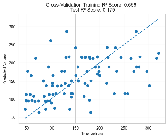
For the best individual, we can use the new features it constructs to train a model. Then, we can transform the test set using these features and evaluate the performance of the model on the test set.
def evaluationOnTest(trees, name):
    # Creating new features
    new_features = []
    for ind_num, ind in enumerate(trees):
        func = gp.compile(expr=ind, pset=pset)
        new_features.append([func(*record) for record in train_X])

    # Transposing the new feature array
    new_features = np.transpose(np.array(new_features))
    model = DecisionTreeRegressor(min_samples_leaf=10)
    model.fit(new_features, train_y)
    train_y_pred = model.predict(new_features)

    # Creating new features
    new_features = []
    for ind_num, ind in enumerate(trees):
        func = gp.compile(expr=ind, pset=pset)
        new_features.append([func(*record) for record in test_X])

    # Transposing the new feature array
    new_features = np.transpose(np.array(new_features))

    # Returning the test error
    score = r2_score(test_y, model.predict(new_features))
    plot_predictions(train_y, train_y_pred, test_y, model.predict(new_features), name)
    return score


evaluationOnTest(best_ind, "Cross-Validation")
GP Directly Optimizing Training Error
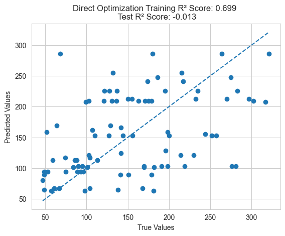
Certainly, we can also use genetic programming to optimize training error directly.
def evalFeatureEngineeringTrainingError(individuals):
    # Creating new features
    new_features = []
    for ind_num, ind in enumerate(individuals):
        func = gp.compile(expr=ind, pset=pset)
        new_features.append([func(*record) for record in train_X])

    # Transposing the new feature array
    new_features = np.transpose(np.array(new_features))

    # Using decision tree for regression
    model = DecisionTreeRegressor(min_samples_leaf=10)
    model.fit(new_features, train_y)

    # Returning the training error
    return r2_score(train_y, model.predict(new_features)),


toolbox.register("evaluate", evalFeatureEngineeringTrainingError)

pop, log = algorithms.eaSimple(population, toolbox, 0.9, 0.1, 10, stats=stats, halloffame=hof, verbose=True)

# Viewing the best individual
best_ind = hof[0]
print('Best individual is:', [str(tree) for tree in best_ind])
print('With fitness:', best_ind.fitness.values)
evaluationOnTest(best_ind, "Direct Optimization")
gen	nevals	avg     	std     	min      	max
0  	0     	0.303931	0.143638	-0.185107	0.45335
1  	88    	0.55985 	0.0987481	0.256506 	0.665762
2  	90    	0.590953	0.0693942	0.267409 	0.682302
3  	86    	0.605792	0.070243 	0.310435 	0.676585
4  	92    	0.599634	0.0660101	0.379885 	0.685347
5  	89    	0.596156	0.0815029	0.301172 	0.684787
6  	94    	0.592179	0.0792609	0.291761 	0.676509
7  	86    	0.599535	0.082606 	0.276139 	0.67517
8  	89    	0.614152	0.0673441	0.376966 	0.699104
9  	91    	0.593205	0.0781903	0.229489 	0.680216
10 	85    	0.608815	0.0651021	0.336586 	0.684946
Best individual is: ['subtract(ARG0, add(ARG1, ARG2))', 'add(ARG8, ARG2)', 'add(subtract(add(ARG6, ARG6), multiply(add(ARG9, ARG0), ARG3)), multiply(ARG6, add(ARG6, ARG0)))']
With fitness: (0.6991039640945576,)
Traditional Feature Engineering Methods
Finally, we can use traditional feature engineering methods such as neural networks and kernel methods to construct new features and then train models to see how they perform.
from sklearn.neural_network import MLPRegressor
from sklearn.svm import SVR

# Using Neural Network
model = MLPRegressor(learning_rate_init=0.01, max_iter=10000)
model.fit(train_X, train_y)
plot_predictions(train_y, model.predict(train_X), test_y, model.predict(test_X), "NN")

# Using Kernel SVM
model = SVR()
model.fit(train_X, train_y)
plot_predictions(train_y, model.predict(train_X), test_y, model.predict(test_X), "KernelSVM")

# Using Decision Tree
model = DecisionTreeRegressor(min_samples_leaf=10)
model.fit(train_X, train_y)
plot_predictions(train_y, model.predict(train_X), test_y, model.predict(test_X), "DT")
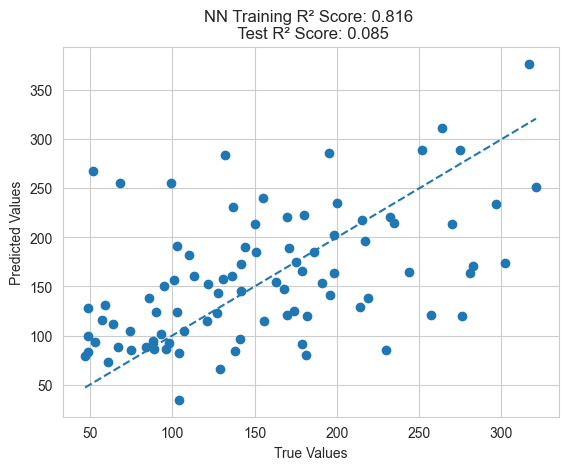
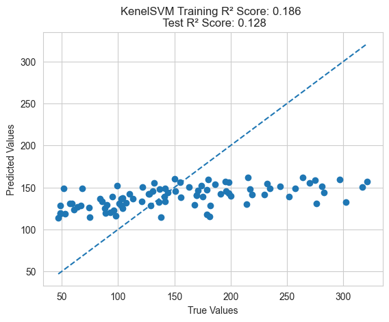
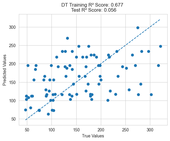
From the above results, it can be seen that the feature engineering method using genetic programming performs better on the test set compared to traditional feature engineering methods. This validates the superiority of GP.
Additionally, it’s important to note that genetic programming feature engineering optimizes cross-validation error rather than directly optimizing training error, resulting in better generalization performance. If training error is directly optimized, it may lead to overfitting and poor generalization to the test set.
